If It Flies ... - 2011/02

February 2011 71
HI, GANG. In the last few columns I wrote about some selected
aspects of glow power, eventually covering the traditional “4-2-4” CL
Precision Aerobatics (Stunt) engine run. Check the film clips that I
mentioned in the December column.
As I wrote, subtly tweaking the engine’s compression ratio, venturi
size, nitro and oil content of the fuel, and even glow-plug heat range
represents one of the high points of classical aeromodeling technique.
Let’s face it; that was downright clever!
This kind of “toy airplane lore” musn’t be allowed to pass into
obscurity, and not because I expect that you’ll use these techniques
directly. You might never fly glow or maybe never CL (a shame, I
think, either way), but it’s important to know about different
techniques, tricks, and methods used in other corners of the
aeromodeling universe. Why? Cross-pollination.
When smart gardeners and farmers cross-pollinate plants or crops,
they often get better, stronger ones. Aeromodeling is like that too!
I have an RC flying buddy who has a neat flying-wing creation. It’s
fairly large and hard to grab for hand launch, not to mention glowpowered.
After a dozen or so scary hand launches, a mutual flying
buddy showed him how to build a wheeled dolly that would securely
cradle the airplane until takeoff and then cleanly drop it off after it
established a climb.
Where did he learn this? CL Speed! Those fliers’ models have
always taken off
from a dolly and
landed on skids.
The Speed pilots
have other tricks,
but that’s for
another day.
Are you cross-pollinating?
Dean Pappas | DeanF3AF2B@If It Flies ... pappasfamily.net
Also included in this column:
• Electric-power control science
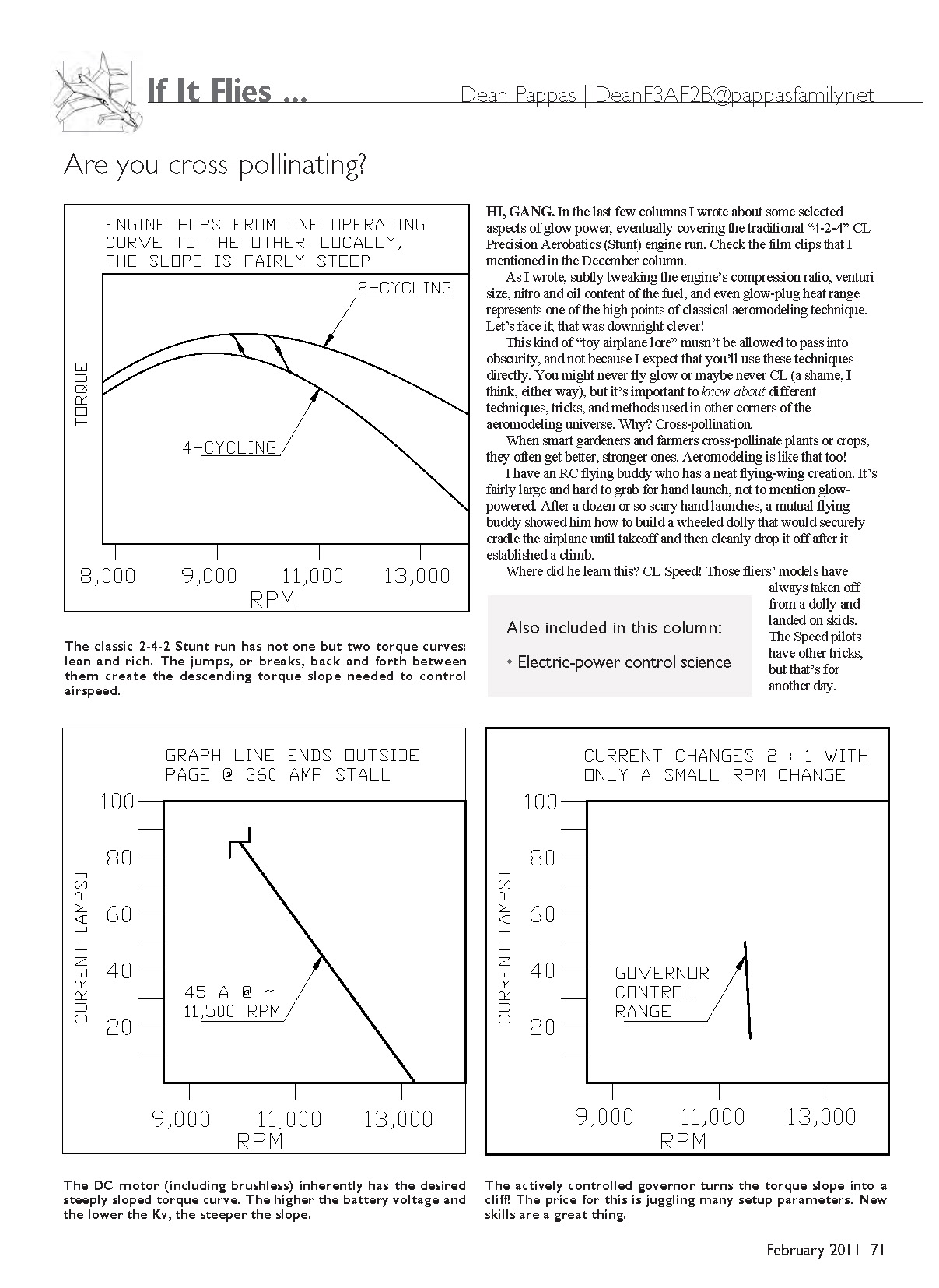
The classic 2-4-2 Stunt run has not one but two torque curves:
lean and rich. The jumps, or breaks, back and forth between
them create the descending torque slope needed to control
airspeed.
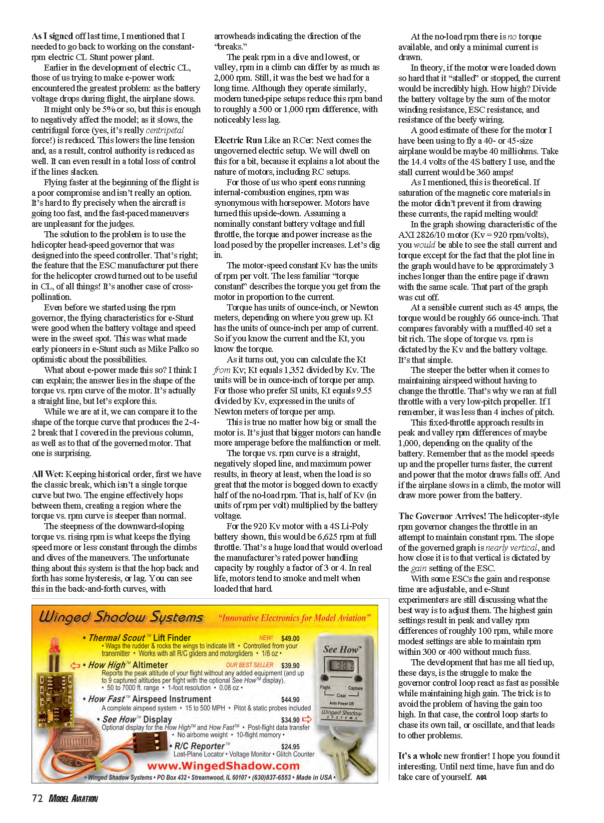
The DC motor (including brushless) inherently has the desired
steeply sloped torque curve. The higher the battery voltage and
the lower the Kv, the steeper the slope.
The actively controlled governor turns the torque slope into a
cliff! The price for this is juggling many setup parameters. New
skills are a great thing.
02sig3.QXD_00MSTRPG.QXD 12/20/10 9:23 AM Page 71
As I signed off last time, I mentioned that I
needed to go back to working on the constantrpm
electric CL Stunt power plant.
Earlier in the development of electric CL,
those of us trying to make e-power work
encountered the greatest problem: as the battery
voltage drops during flight, the airplane slows.
It might only be 5% or so, but this is enough
to negatively affect the model; as it slows, the
centrifugal force (yes, it’s really centripetal
force!) is reduced. This lowers the line tension
and, as a result, control authority is reduced as
well. It can even result in a total loss of control
if the lines slacken.
Flying faster at the beginning of the flight is
a poor compromise and isn’t really an option.
It’s hard to fly precisely when the aircraft is
going too fast, and the fast-paced maneuvers
are unpleasant for the judges.
The solution to the problem is to use the
helicopter head-speed governor that was
designed into the speed controller. That’s right;
the feature that the ESC manufacturer put there
for the helicopter crowd turned out to be useful
in CL, of all things! It’s another case of crosspollination.
Even before we started using the rpm
governor, the flying characteristics for e-Stunt
were good when the battery voltage and speed
were in the sweet spot. This was what made
early pioneers in e-Stunt such as Mike Palko so
optimistic about the possibilities.
What about e-power made this so? I think I
can explain; the answer lies in the shape of the
torque vs. rpm curve of the motor. It’s actually
a straight line, but let’s explore this.
While we are at it, we can compare it to the
shape of the torque curve that produces the 2-4-
2 break that I covered in the previous column,
as well as to that of the governed motor. That
one is surprising.
All Wet: Keeping historical order, first we have
the classic break, which isn’t a single torque
curve but two. The engine effectively hops
between them, creating a region where the
torque vs. rpm curve is steeper than normal.
The steepness of the downward-sloping
torque vs. rising rpm is what keeps the flying
speed more or less constant through the climbs
and dives of the maneuvers. The unfortunate
thing about this system is that the hop back and
forth has some hysteresis, or lag. You can see
this in the back-and-forth curves, with
arrowheads indicating the direction of the
“breaks.”
The peak rpm in a dive and lowest, or
valley, rpm in a climb can differ by as much as
2,000 rpm. Still, it was the best we had for a
long time. Although they operate similarly,
modern tuned-pipe setups reduce this rpm band
to roughly a 500 or 1,000 rpm difference, with
noticeably less lag.
Electric Run Like an RCer: Next comes the
ungoverned electric setup. We will dwell on
this for a bit, because it explains a lot about the
nature of motors, including RC setups.
For those of us who spent eons running
internal-combustion engines, rpm was
synonymous with horsepower. Motors have
turned this upside-down. Assuming a
nominally constant battery voltage and full
throttle, the torque and power increase as the
load posed by the propeller increases. Let’s dig
in.
The motor-speed constant Kv has the units
of rpm per volt. The less familiar “torque
constant” describes the torque you get from the
motor in proportion to the current.
Torque has units of ounce-inch, or Newton
meters, depending on where you grew up. Kt
has the units of ounce-inch per amp of current.
So if you know the current and the Kt, you
know the torque.
As it turns out, you can calculate the Kt
from Kv; Kt equals 1,352 divided by Kv. The
units will be in ounce-inch of torque per amp.
For those who prefer SI units, Kt equals 9.55
divided by Kv, expressed in the units of
Newton meters of torque per amp.
This is true no matter how big or small the
motor is. It’s just that bigger motors can handle
more amperage before the malfunction or melt.
The torque vs. rpm curve is a straight,
negatively sloped line, and maximum power
results, in theory at least, when the load is so
great that the motor is bogged down to exactly
half of the no-load rpm. That is, half of Kv (in
units of rpm per volt) multiplied by the battery
voltage.
For the 920 Kv motor with a 4S Li-Poly
battery shown, this would be 6,625 rpm at full
throttle. That’s a huge load that would overload
the manufacturer’s rated power handling
capacity by roughly a factor of 3 or 4. In real
life, motors tend to smoke and melt when
loaded that hard.
72 MODEL AVIATION
At the no-load rpm there is no torque
available, and only a minimal current is
drawn.
In theory, if the motor were loaded down
so hard that it “stalled” or stopped, the current
would be incredibly high. How high? Divide
the battery voltage by the sum of the motor
winding resistance, ESC resistance, and
resistance of the beefy wiring.
A good estimate of these for the motor I
have been using to fly a 40- or 45-size
airplane would be maybe 40 milliohms. Take
the 14.4 volts of the 4S battery I use, and the
stall current would be 360 amps!
As I mentioned, this is theoretical. If
saturation of the magnetic core materials in
the motor didn’t prevent it from drawing
these currents, the rapid melting would!
In the graph showing characteristic of the
AXI 2826/10 motor (Kv = 920 rpm/volts),
you would be able to see the stall current and
torque except for the fact that the plot line in
the graph would have to be approximately 3
inches longer than the entire page if drawn
with the same scale. That part of the graph
was cut off.
At a sensible current such as 45 amps, the
torque would be roughly 66 ounce-inch. That
compares favorably with a muffled 40 set a
bit rich. The slope of torque vs. rpm is
dictated by the Kv and the battery voltage.
It’s that simple.
The steeper the better when it comes to
maintaining airspeed without having to
change the throttle. That’s why we ran at full
throttle with a very low-pitch propeller. If I
remember, it was less than 4 inches of pitch.
This fixed-throttle approach results in
peak and valley rpm differences of maybe
1,000, depending on the quality of the
battery. Remember that as the model speeds
up and the propeller turns faster, the current
and power that the motor draws falls off. And
if the airplane slows in a climb, the motor will
draw more power from the battery.
The Governor Arrives! The helicopter-style
rpm governor changes the throttle in an
attempt to maintain constant rpm. The slope
of the governed graph is nearly vertical, and
how close it is to that vertical is dictated by
the gain setting of the ESC.
With some ESCs the gain and response
time are adjustable, and e-Stunt
experimenters are still discussing what the
best way is to adjust them. The highest gain
settings result in peak and valley rpm
differences of roughly 100 rpm, while more
modest settings are able to maintain rpm
within 300 or 400 without much fuss.
The development that has me all tied up,
these days, is the struggle to make the
governor control loop react as fast as possible
while maintaining high gain. The trick is to
avoid the problem of having the gain too
high. In that case, the control loop starts to
chase its own tail, or oscillate, and that leads
to other problems.
It’s a whole new frontier! I hope you found it
interesting. Until next time, have fun and do
take care of yourself. MA
02sig3.QXD_00MSTRPG.QXD 12/20/10 9:23 AM Page 72